SDCD: Simulated Data for Concept Drift

Developed for project: #EP/D0404X/1 Classifier Ensembles for Changing Environments
Sponsored by EPSRC.
(related keywords: concept drift, population drift, hidden contexts, recurring contexts)

A fundamental assumption often made in supervised classification is that the problem is static, i.e., the description of the classes does not change with time. However many practical classification tasks involve changing environments. Thus designing and testing classifiers for changing environments are of increasing interest and importance. A number of benchmark data sets are available for static classification tasks. For example, the UCI machine learning repository is extensively used by researchers to compare algorithms across various domains. Only few benchmark datasets are available for changing environments. Also, while generating data for static environments is relatively straightforward, this is not so for changing environments. The reason is that an infinite amount of changes can be simulated, and it is difficult to define which ones will be realistic and hence useful. We proposed a general framework for generating data to simulate changing environments in:

Narasimhamurthy A., L.I. Kuncheva, A framework for generating data to simulate changing environments, Proc. IASTED, Artificial Intelligence and Applications, Innsbruck, Austria, 2007, 384-389. pdf [bib]

Content

1. simulation_changing_environment.m

[A,LABA] = simulation_changing_environment(P, V)

returns a data set A with N points and a label vector LABA. V is an array with probabilities of size N-by-K, where K is the number of sources to sample from. The rows of V, V(i,:) are the mixing proportions of the K sources (each row of V sums up to 1). P is a user-defined function called as [X,LABX] = P(i), which samples once from data source i and returns point X with its label. The programme implements the following algorithm:

I. Initialise the data set A = empty and the set of labels LABA = empty.
II. For i = 1,...,N
(i). k = Sample once from the set {1,2,...,K} with distribution defined by V(i,1),...,V(i,K) to determine which of the K sources will provide the next point.
(ii). Sample a new data point from source k, [x,labx] = P(k) and add x to the current set A. Add the class label labx to LABA.
III. End i
IV. Return data set A and labels LABA.
2. p_stagger.m

[x,labx] = p_stagger(k)

Samples one point (=instance, =example) from the STAGGER data problem, widely used as a benchmark artificial dataset for changing environments. The feature space is described by three features (attributes): size {small, medium, large}, colour {red, green, blue} and shape {square, circular, triangular}. There are three data sources (called target concepts):

Target Concept 1 : size = small AND color = red
Target Concept 2 : color = green OR shape = circular
Target Concept 3 : size = medium OR size = large

In their experiment, Widmer and Kubat [1] generate randomly 120 training instances and label each instance according to the current target concept. After processing each instance, the predictive accuracy is tested on an independent test set of 100 instances, also generated randomly. One target concept is active at a time. Concept 1 is active from instance 1 to instance 40, Concept 2 is active from instance 41 to 80 and Concept 3 from instance 81 to 120.

All you need to do in order to generate a training set A with labels LABA sampled from the STAGGER distribution is the following couple of lines:

V = [repmat([1 0 0],40,1);repmat([0 1 0],40,1);repmat([0 0 1],40,1)];
[A,LABA] = simulation_changing_environment('p_stagger',V);

The values of each of the 3 features are coded with integers 1, 2 and 3. For example [2,3,2] denotes (medium size, blue colour, triangular shape). The code for generating a training set of 120 STAGGER data points is also available as STAGGER_training_data.m
3. p_hyperplane2d.m

[x,labx] = p_hyperplane2d(k)

This function can be used as input in simulation_changing_environment in order to generate the "moving hyperplane data" in 2d, often used as benchmark. Point x returned by the function lies in the square [-1,+1]-by-[-1,+1]. There are two classes with equal prior probabilities. The data on one side of the hyperplane are labelled as class 1 and on the other side as class 2. If static data is required, the programme should be called in a loop with a fixed angle k of the separating plane. For changing environments k may be varied as desired. For this example we assume that there are 360 data sources determined by the degree of rotation of the separating line. The code Moving_hyperplane_2d_demo.m shows an animation of the generated data as the line rotates in full circle.
4. p_gaussian2d_4components.m

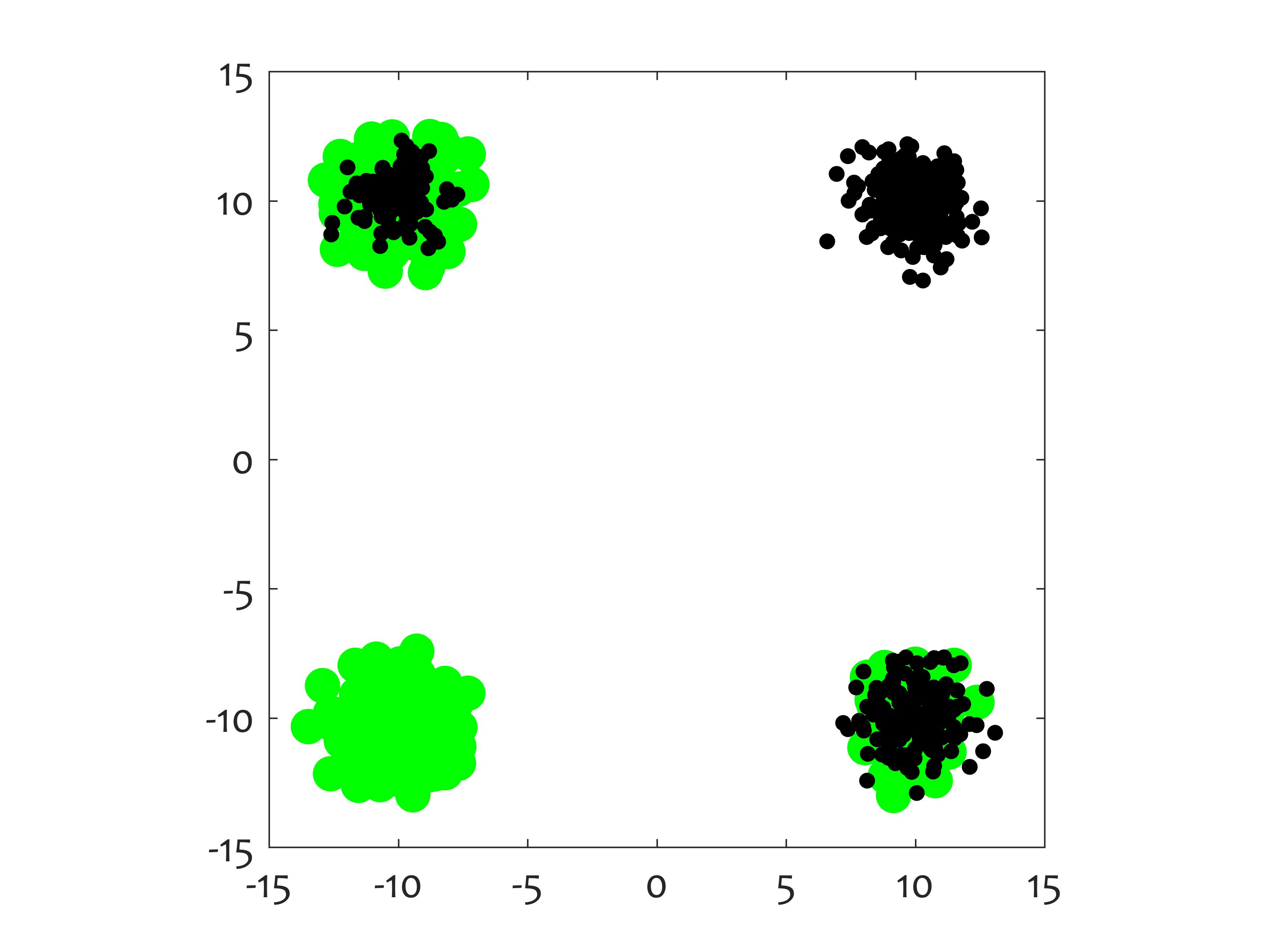
[x,labx] = p_gaussian2d_4components(k,s)

This function can be used in simulation_changing_environment. It samples a point from a 2-dimensional mixture of 4 equiprobable Gaussian clusters, and labels the point into one of 2 classes. There are two concepts, so k = 1 or 2. "s" is an optional parameter specifying the variance of all clusters. Suppose that point x has coordinates (x1,x2). According to the first concept, if x2 is negative, the class label of x is 1, otherwise the class label is 2. According to the second concept, x is labelled as class 1 if x1 is negative, and in class 2 otherwise. Gaussian_2d_demo.m shows an animation of the generated data as one of the concepts fades away and is replaced by the other concept.
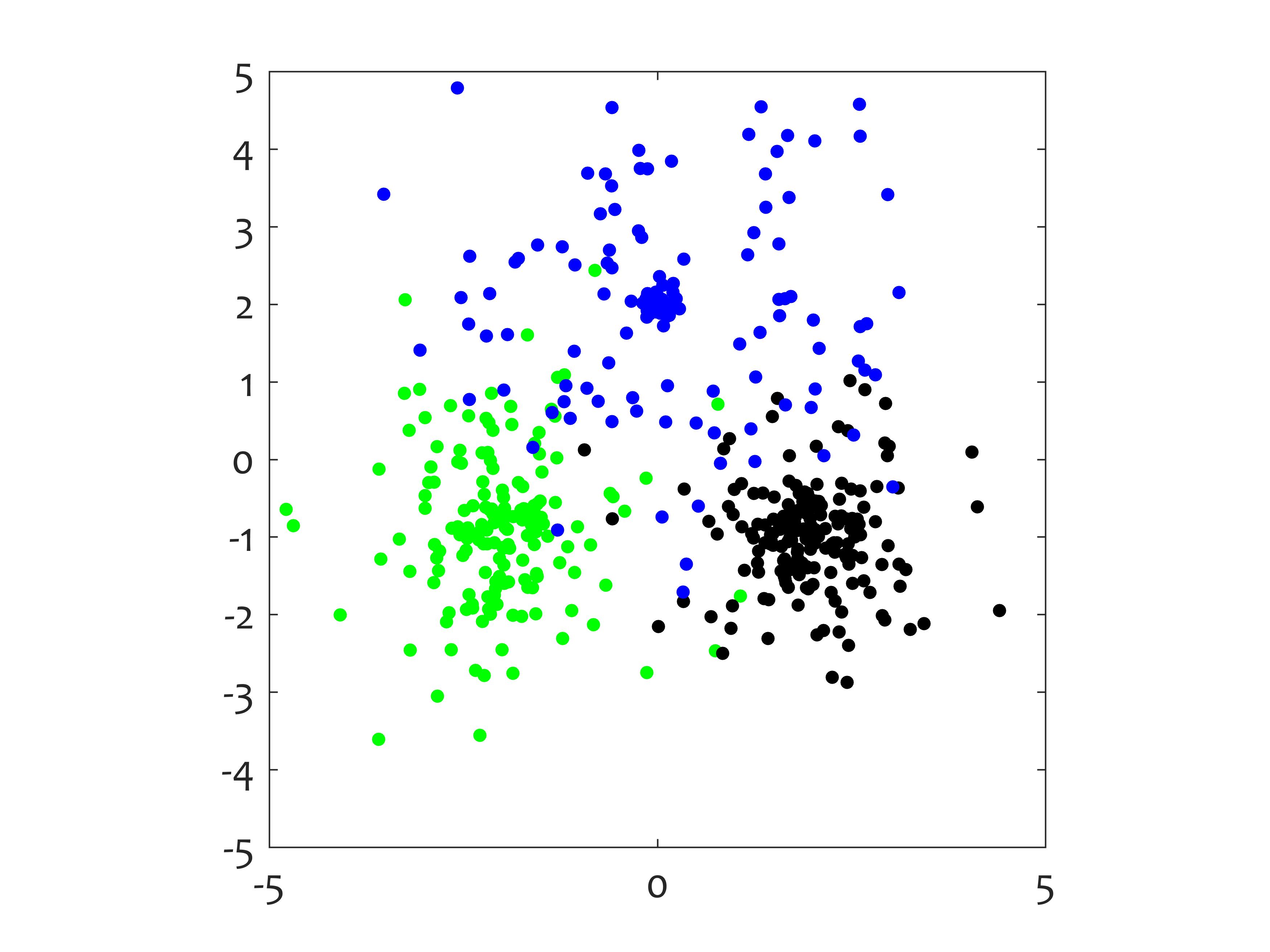
5. p_gaussians_3class_changing_variance.m

[x,labx] = p_gaussians_3class_changing_variance(k,n)

This function can be used in simulation_changing_environment. It samples a point from 3 Gaussian classes with static means and changing variances. The means of the first two components are at [-2 -1], [2 -1] and [0 2], respectively. The remaining n-2 components have means 0. (If n is not specified, the default value n = 2 is used.) The covariance matrices are diagonal. The variances of the first two features are varied but are kept equal within each cluster. The classes are equiprobable. There are 5 concepts corresponding to the following sets of standard deviations for the three classes:

s1 s2 s3

1: 1.4 1.1 0.1

2: 0.6 0.4 1.7

3: 1.3 1.3 0.9

4: 0.3 0.3 0.1

5: 1.6 0.3 1.4

Gaussian_3class_demo.m shows an animation of the generated data as one of the concepts fades away and is replaced by the next one in the list.

	s1	s2	s3
1:	1.4	1.1	0.1
2:	0.6	0.4	1.7
3:	1.3	1.3	0.9
4:	0.3	0.3	0.1
5:	1.6	0.3	1.4

	s1	s2	s3
1:	1.4	1.1	0.1
2:	0.6	0.4	1.7
3:	1.3	1.3	0.9
4:	0.3	0.3	0.1
5:	1.6	0.3	1.4

	s1	s2	s3
1:	1.4	1.1	0.1
2:	0.6	0.4	1.7
3:	1.3	1.3	0.9
4:	0.3	0.3	0.1
5:	1.6	0.3	1.4